很早就想梳理一下关于Diffusion Model的相关知识，试图不再“畏惧”那一大堆数学公式

本文将基于Google Research, Brain Team在2022年的一篇综述文章《Understanding Diffusion Models: A Unified Perspective》https://arxiv.org/abs/2208.11970 ，逐步展开理解DDPM、DDIM等Diffusion Models所需要的一些数学知识。

生成式模型

Given observed samples $x$ from a distribution of interest, the goal of a generative model is to learn to model its true data distribution $p(x)$. Once learned, we can generate new samples from our approximate model at will. Furthermore, under some formulations, we are able to use the learned model to evaluate the likelihood of observed or sampled data as well.

这一段话给出了生成式模型的一个定义，即“从样本数据分布中学习到真实数据分布，并可以从学习到的真实数据分布中采样出新的样本”。这里的从样本数据分布中学习到真实数据分布，其实也就是数理统计中参数估计的过程，因为我们通常会假设真实数据分布满足一个高斯分布律，那么从样本数据分布中学习到真实数据分布也就是对这个高维高斯分布的参数进行估计的过程。

There are several well-known directions in current literature, that we will only introduce briefly at a high level. Generative Adversarial Networks (GANs) model the sampling procedure of a complex distribution, which is learned in an adversarial manner. Another class of generative models, termed "likelihood-based", seeks to learn a model that assigns a high likelihood to the observed data samples. This includes autoregressive models, normalizing flows, and Variational Autoencoders (VAEs). Another similar approach is energy-based modeling, in which a distribution is learned as an arbitrarily flexible energy function that is then normalized.

这里提到GAN与VAE两种方法，GAN（生成对抗网络）是利用了对抗的方法对采样过程进行建模，用一个神经网络直接去拟合真实分布，优化目标是使得真实数据分布与生成数据分布的KL散度达到最小。

而VAE则是基于极大似然估计的方法，神经网络的优化目标是使得样本数据分布出现的概率最大。

这里只是给出了定性的理解，并没有给出公式（真要写公式还挺复杂的hhh）

Score-based generative models are highly related; instead of learning to model the energy function itself, they learn the score of the energy-based model as a neural network. In this work we explore and review diffusion models, which as we will demonstrate, have both likelihood-based and score-based interpretations. We showcase the math behind such models in excruciating detail, with the aim that anyone can follow along and understand what diffusion models are and how they work.

这里提及了一下score-based模型，对于score-based方法，我并不是太了解，不过diffusion model是可以从likelihood-based与score-based两种角度解读的。其中DDPM的原论文就是通过likelihood-based方法推导公式，而Score-Based Generative Modeling through Stochastic Differential Equations(arxiv: https://arxiv.org/abs/2011.13456) 则是通过随机微分方程（SDE）的方式完成了score-based的角度解读。

从AutoEncoder开始

在wikipedia上，https://en.wikipedia.org/wiki/Autoencoder ,AE的作用是学习对高维度数据做低维度“表示”（“表征”或“编码”）；因此，通常用于降维。利用AE学习到的encoder对数据进行编码，将$x$（一般是图片）从高维空间$\mathbb{R}^{w\times h}$编码（降维）到latent code $z$（一个特征向量）低维空间$\mathbb{R}^{n}$，一般$n\ll w\times h$。

这实际上包含一种洞见，即我们所看到的样本数据，实际包含了大量的冗余信息。我们实际上可以通过寻找样本空间$\mathcal{X}$的一个子空间$\mathcal{Z}$，即构造一个映射$E_{\phi }:\mathcal {X}\rightarrow \mathcal {Z}$，完成对高维度数据做低维度“表示”。其中映射$E_{\phi }$称作编码器，$\phi$为该编码器的参数。

为了找到这个编码器$E_{\phi }$，我们有多种方法，但归根结底都可以表示成对proxy task的优化。例如，我们可以假设将该编码器$E_{\phi }$所得到的latent code $z$用于图像分类任务应该具有较好的表现，也就是说将proxy task设置为image classification。那么我们可以构造一个分类器$D_{\theta }:\mathcal {Z}\rightarrow \mathcal {L}$，其中$\mathcal {L}$为预测label的取值空间。为了优化这个proxy task，我们使用梯度下降法对样本label真实分布$\hat{\mathcal{L}}$与预测label的取值分布$\mathcal{L}$的交叉熵进行优化，也就是

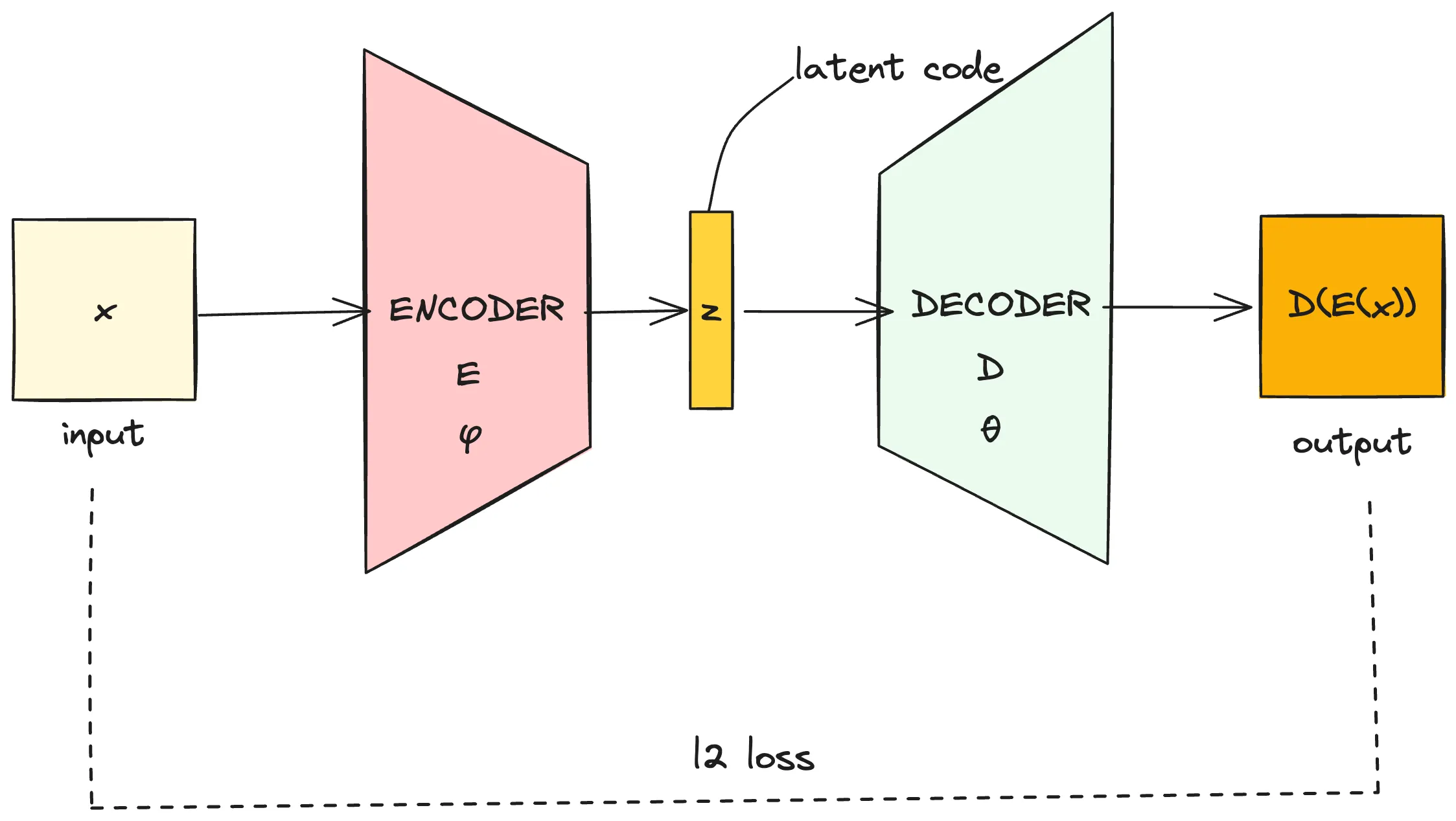
对于AutoEncoder，最理想的proxy task是完全恢复输入的样本信息，也就是无损降维。具体来说，我们期望映射$D_{\theta }$可以完成$D_{\theta }:\mathcal {Z}\rightarrow \mathcal {X}$，将latent code $z$重新恢复为$E_{\phi }$输入的$x$。为了优化这个reconstruction task，我们一般使用L2损失，也即

使用神经网络作为编码器与解码器，那么AE可以用下图(使用excalidraw绘制)表示

VAE——变分自编码器

VAE的原论文是Auto-Encoding Variational Bayes(arxiv: https://arxiv.org/abs/1312.6114v11)

首先我们看看VAE的网络架构 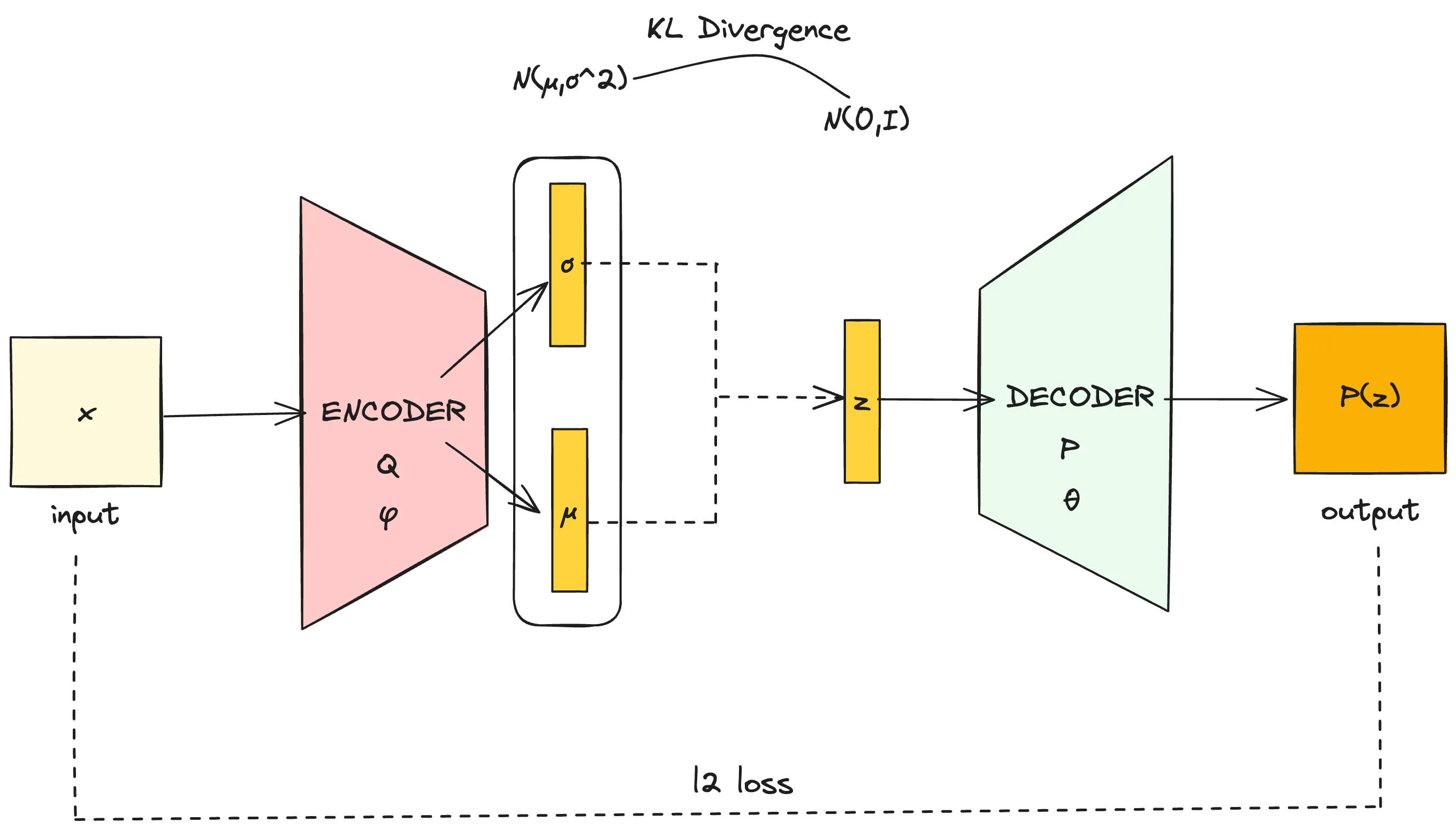这个网络结构跟AE基本完全一样，只是Encoder部分的输出是一组$\sigma$参数与$\mu$参数，从由这两个参数决定的高斯分布$\mathcal{N}(\mu,\sigma^2)$中采样出隐变量$z$作为decoder的输入。损失函数部分，除了L2损失以外额外加入了分布$\mathcal{N}(\mu,\sigma^2)$对分布$\mathcal{N}(0,I)$的KL散度。

首先，可以肯定的是，VAE与AE之间肯定会存在着十分紧密的关系。但我们会想，VAE将encoder直接编码隐变量$z$变为encoder输出一个高斯分布，从高斯分布中采样一个隐变量是为了什么呢？

让我们回到生成式模型的目标，生成式模型的目标是从估计的真实数据分布中采样得到新的样本，也就是说，当我们确定隐变量$z$满足的分布$p(z)$时，从$p(z)$中任意采样一个$z$，经过decoder得到的$p(x|z)$都应该是有意义的新样本。通俗来说，这要求我们任取一个$z$，decoder都能恢复出一个清晰的有意义的图像。而AE模型则无法完成上述要求，从实验结果来看，对于随机采样的一个$z$，AE的decoder恢复出的图像大多是模糊的无意义的乱码。这是因为由于只存在L2重建损失且encoder直接完成对隐变量$z$的编码，$z$的分布$p(z)$会被过度压缩（过度降维），导致$p(z)$只分布在一个很小的流形上。而在$p(z)$之外的随机采样则无法获得有效的重建结果。

为了解决上述不足，VAE做出了一个先验假设，即隐变量$z$的分布$p(z)\sim\mathcal{N}(0,I)$，或记作$p(z)=\mathcal{N}(z;0,I)$。并让encoder完成对$z$分布的点估计。

我们记encoder为$q_\phi(z|x)$，表示给定$x$的条件下，$z$的估计分布。decoder为$p_\theta(x|z)$，表示给定$z$的条件下，$x$的估计分布。

回忆生成式模型的优化目标，我们要使得样本数据分布出现的概率最大。即使得$p(x)$最大。采用极大对数似然法，优化目标可以写作$\log p(x)$

由于

我们记$\mathbb{E}_{q_\phi(z|x)}\left[\log \frac{p(x,z)}{q_\phi(z|x)} \right]$为ELBO（Evidence Lower Bound）。

下面将说明，对ELBO的优化，也即是对$\log p(x)$下界的优化，是一个合适的proxy optimization objective。

由于$\log p(x)=\mathbb{E}_{q_\phi(z|x)}\left[\log \frac{p(x,z)}{q_\phi(z|x)} \right]+D_{KL}(q_\phi(z|x)||p(z|x))$，注意这里的$p(x)$、$p(x,z)$、$p(z|x)$都是真实分布，是一个固定的分布，整个优化目标可以写作

当调整$\phi$时，总能通过优化ELBO使得$D_{KL}(q_\phi(z|x)||p(z|x))=0$，这样ELBO就达到$\log p(x)$这一上界。

上述过程称作变分贝叶斯估计（Variational Bayes）。

下面，我们将引入解码器$p_\theta(x|z)$作为对$p(x|z)$的估计。

称$\mathbb{E}_{q_\phi(z|x)}\left[\log p_\theta(x|z) \right]$为重建项，$D_{KL}(q_\phi(z|x)||p(z))$为先验匹配项。那么，优化ELBO也就是使得重建项尽量大而先验匹配项尽量小。具体来说，也就是让$q_\phi(z|x)$与$p(z)$的分布尽量靠近，前面我们提到，$p(z)$的分布我们假设是服从$p(z)\sim\mathcal{N}(0,I)$。而重建项的含义为，在给定$q_\phi(z|x)$的情况下（encoder已经完成编码），$p_\theta(x|z)$的值要尽量的大（decoder要尽量恢复重建出$x$）

现在，我们可以理解VAE的网络结构图了，在AE的基础上，让encoder输出一组均值与方差，使得$q_\phi(z|x)$尽量与$p(z)=\mathcal{N}(z;0,I)$靠近，而给定$x$时，通过$q_\phi(z|x)$得到隐变量$z$，使用decoder完成图像重建，并使用L2损失。

HVAE